1. 扩散模型简介
扩散模型(Diffusion Model)是深度生成模型中的SOTA,相比于GAN、VAE、Flow-based这些生成模型而言,扩散模型可以取得更好的效果。扩散模型受非平衡热力学启发,它定义了一条多时间步的马尔可夫链来逐步给图片添加噪声,如果时间步够大,最终图片会变成纯噪声,扩散模型的目的是学习反向的扩散过程,也就是输入随机噪声,能返回一张图片,相比于之前提到的各种生成模型而言,扩散模型具有相对固定的学习步骤,同时隐变量维度更高(和输入数据同样的维度)
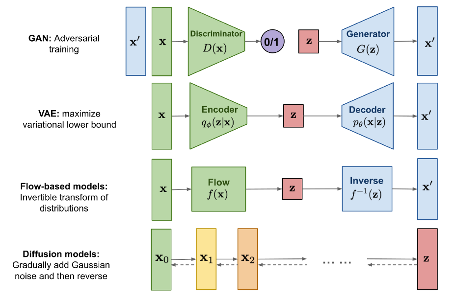
扩散模型的早在2015年便提出了(论文链接),但在当时没有引起广泛的关注,直到2019年NCSN和2020年DDPM的出现才将扩散模型引入了新高度,2022年火爆的text2image模型GLIDE、DALLE2、Latent Diffusion、Imagen的相继提出,让扩散模型火出了圈,这篇博客将对扩散模型的前向计算、反向训练、训练、生成步骤及其数学原理做详细的整理,会列出很多数学公式,同时该博客也参考了很多相关资料,这里我一并列出
2. 模型
2.1. 前向扩散
从原始数据分布中采样$x_0$, 假设$x_0\sim q(x)$,前向扩散过程就是在每一个时间步都加上一个高斯噪声,这样就可以从最初的$x_0$生成长度为T的噪声序列$x_1, x_2, x_3,…, x_T$,每一步都用variance schedule$\beta_t$控制,其中$\beta_t\in (0, 1)$,每一步的后验分布(预定义好的)为:
\begin{equation}
q(\mathbf{x}_t \vert \mathbf{x}_{t-1}) = \mathcal{N}(\mathbf{x}_t; \sqrt{1 - \beta_t} \mathbf{x}_{t-1}, \beta_t\mathbf{I}) \quad
q(\mathbf{x}_{1:T} \vert \mathbf{x}_0) = \prod^T_{t=1} q(\mathbf{x}_t \vert \mathbf{x}_{t-1})
\end{equation}
这个前向传播的过程中有一个非常好的性质,就是我们可以在任意时间步采样得到$x_t$,为了实现这个技巧,我们需要用到reparameterization技巧(该技巧也在VAE中出现过),重参数化技巧的本质就是将随机采样的z通过引入高斯噪声$\epsilon$变成确定性的z,也就是上面的$x_t$可以表示为$x_t=\sqrt{1-\beta_t}x_{t-1}+\sqrt{\beta_t}\epsilon$,这样有利于梯度的逆传播,那么我们可以推出以下公式:
\begin{equation}
\begin{aligned}
\mathbf{x}_t
&= \sqrt{\alpha_t}\mathbf{x}_{t-1} + \sqrt{1 - \alpha_t}\boldsymbol{\epsilon}_{t-1} \\
&= \sqrt{\alpha_t \alpha_{t-1}} \mathbf{x}_{t-2} + \sqrt{1 - \alpha_t \alpha_{t-1}} \bar{\boldsymbol{\epsilon}}_{t-2} \\
&= \dots \\
&= \sqrt{\bar{\alpha}_t}\mathbf{x}_0 + \sqrt{1 - \bar{\alpha}_t}\boldsymbol{\epsilon} \\
q(\mathbf{x}_t \vert \mathbf{x}_0) &= \mathcal{N}(\mathbf{x}_t; \sqrt{\bar{\alpha}_t} \mathbf{x}_0, (1 - \bar{\alpha}_t)\mathbf{I})
\end{aligned}
\end{equation}
其中$\epsilon_t$都是均值为0,方差为1的高斯噪声,$\alpha_t=1-\beta_t$, $\bar{\alpha_t}=\prod_{i=1}^t\alpha_i$, 注:两个均值相同高斯噪声可以合并成一个高斯噪声,方差为之前方差的平方和开根号,一般来说,$\beta_1<\beta_2<…<\beta_T$
2.2. 反向扩散过程
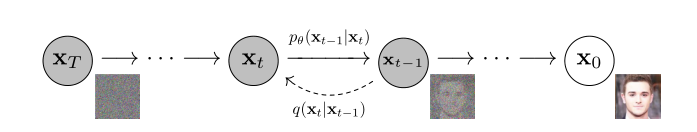
如果我们可以将前向传播的过程反向,那么我们就可以获得后验分布$q(x_{t-1}|x_{t})$,那么我们就可以利用马尔科夫链的性质,输入高斯噪声,然后获得生成的照片,但是,我们无法高效地得到$q(x_{t-1}|x_{t})$,于是我们希望学习出分布$p_\theta$来模拟后验分布$q(x_{t-1}|x_{t})$,由于前向扩散的过程中我们假设后验分布是高斯分布,所以这里我们也假设$p_\theta$是高斯分布,于是我们有:
\begin{equation}
p_\theta(\mathbf{x}_{0:T}) = p(\mathbf{x}_T) \prod^T_{t=1} p_\theta(\mathbf{x}_{t-1} \vert \mathbf{x}_t) \quad
p_\theta(\mathbf{x}_{t-1} \vert \mathbf{x}_t) = \mathcal{N}(\mathbf{x}_{t-1}; \boldsymbol{\mu}_\theta(\mathbf{x}_t, t), \boldsymbol{\Sigma}_\theta(\mathbf{x}_t, t))
\end{equation}
其中分布$p_\theta$中的均值$\mu$和方差$\Sigma$与时间步t和输入$x_t$有关
虽然我们不知道$q(x_{t-1}|x_t)$的分布情况,但是我们可以知道$q(\mathbf{x}_{t-1} \vert \mathbf{x}_t, \mathbf{x}_0)$的分布情况,推导过程如下:
\begin{equation}
\begin{aligned}
q\left(\mathbf{x}_{t-1} \mid \mathbf{x}_t, \mathbf{x}_0\right) &=q\left(\mathbf{x}_t \mid \mathbf{x}_{t-1}, \mathbf{x}_0\right) \frac{q\left(\mathbf{x}_{t-1} \mid \mathbf{x}_0\right)}{q\left(\mathbf{x}_t \mid \mathbf{x}_0\right)} \\
& \propto \exp \left(-\frac{1}{2}\left(\frac{\left(\mathbf{x}_t-\sqrt{\alpha_t} \mathbf{x}_{t-1}\right)^2}{\beta_t}+\frac{\left(\mathbf{x}_{t-1}-\sqrt{\bar{\alpha}_{t-1}} \mathbf{x}_0\right)^2}{1-\bar{\alpha}_{t-1}}-\frac{\left(\mathbf{x}_t-\sqrt{\bar{\alpha}_t} \mathbf{x}_0\right)^2}{1-\bar{\alpha}_t}\right)\right) \\
&=\exp \left(-\frac{1}{2}\left(\frac{\mathbf{x}_t^2-2 \sqrt{\alpha_t} \mathbf{x}_t \mathbf{x}_{t-1}+\alpha_t \mathbf{x}_{t-1}^2}{\beta_t}+\frac{\mathbf{x}_{t-1}^2-2 \sqrt{\bar{\alpha}_{t-1}} \mathbf{x}_0 \mathbf{x}_{t-1}+\bar{\alpha}_{t-1} \mathbf{x}_0^2}{1-\bar{\alpha}_{t-1}}-\frac{\left(\mathbf{x}_t-\sqrt{\bar{\alpha}_t} \mathbf{x}_0\right)^2}{1-\bar{\alpha}_t}\right)\right) \\
&=\exp \left(-\frac{1}{2}\left(\left(\frac{\alpha_t}{\beta_t}+\frac{1}{1-\bar{\alpha}_{t-1}}\right) \mathbf{x}_{t-1}^2-\left(\frac{2 \sqrt{\alpha_t}}{\beta_t} \mathbf{x}_t+\frac{2 \sqrt{\bar{\alpha}_{t-1}}}{1-\bar{\alpha}_{t-1}} \mathbf{x}_0\right) \mathbf{x}_{t-1}+C\left(\mathbf{x}_t, \mathbf{x}_0\right)\right)\right)
\end{aligned}
\end{equation}
其中函数$C(x_t, x_0)$与$x_{t-1}$无关,根据上述式子我们可以得出$q(x_{t-1}|x_t,x_0)$满足正态分布,均值和标准差分别为$\tilde{\mu_t}$和$\tilde{\beta_t}$,表达式分别为:
\begin{equation}
\begin{aligned}
\tilde{\beta}_t
&= 1/(\frac{\alpha_t}{\beta_t} + \frac{1}{1 - \bar{\alpha}_{t-1}})
= 1/(\frac{\alpha_t - \bar{\alpha}_t + \beta_t}{\beta_t(1 - \bar{\alpha}_{t-1})})
= \frac{1 - \bar{\alpha}_{t-1}}{1 - \bar{\alpha}_t} \cdot \beta_t \\
\tilde{\boldsymbol{\mu}}_t (\mathbf{x}_t, \mathbf{x}_0)
&= (\frac{\sqrt{\alpha_t}}{\beta_t} \mathbf{x}_t + \frac{\sqrt{\bar{\alpha}_{t-1} }}{1 - \bar{\alpha}_{t-1}} \mathbf{x}_0)/(\frac{\alpha_t}{\beta_t} + \frac{1}{1 - \bar{\alpha}_{t-1}}) \\
&= (\frac{\sqrt{\alpha_t}}{\beta_t} \mathbf{x}_t + \frac{\sqrt{\bar{\alpha}_{t-1} }}{1 - \bar{\alpha}_{t-1}} \mathbf{x}_0) \frac{1 - \bar{\alpha}_{t-1}}{1 - \bar{\alpha}_t} \cdot \beta_t \\
&= \frac{\sqrt{\alpha_t}(1 - \bar{\alpha}_{t-1})}{1 - \bar{\alpha}_t} \mathbf{x}_t + \frac{\sqrt{\bar{\alpha}_{t-1}}\beta_t}{1 - \bar{\alpha}_t} \mathbf{x}_0\\
\end{aligned}
\end{equation}
于是最终可以得到$q(x_{t-1}|x_t,x_0)$:
\begin{equation}
q(\mathbf{x}_{t-1} \vert \mathbf{x}_t, \mathbf{x}_0) = \mathcal{N}(\mathbf{x}_{t-1}; \tilde{\boldsymbol{\mu}}(\mathbf{x}_t, \mathbf{x}_0), \tilde{\beta}_t \mathbf{I})
\end{equation}
在根据马尔可夫链我们有: $\mathbf{x}_0 = \frac{1}{\sqrt{\bar{\alpha}_t}}(\mathbf{x}_t - \sqrt{1 - \bar{\alpha}_t}\boldsymbol{\epsilon}_t)$,注意这里的$\epsilon_t$并不是任意的一个噪声,而是让$x_0$变成$x_t$的噪声,那么$\tilde{\mu_t}$可以表示为:
\begin{equation}
\begin{aligned}
\tilde{\boldsymbol{\mu}}_t
&= \frac{\sqrt{\alpha_t}(1 - \bar{\alpha}_{t-1})}{1 - \bar{\alpha}_t} \mathbf{x}_t + \frac{\sqrt{\bar{\alpha}_{t-1}}\beta_t}{1 - \bar{\alpha}_t} \frac{1}{\sqrt{\bar{\alpha}_t}}(\mathbf{x}_t - \sqrt{1 - \bar{\alpha}_t}\boldsymbol{\epsilon}_t) \\
&= \frac{1}{\sqrt{\alpha_t}} \Big( \mathbf{x}_t - \frac{1 - \alpha_t}{\sqrt{1 - \bar{\alpha}_t}} \boldsymbol{\epsilon}_t \Big)
\end{aligned}
\end{equation}
2.3. 损失函数
和VAE类似,也可以用Variational Lower Bound来最大边缘似然函数$p_\theta(x_0)$:
\begin{equation}
\begin{aligned}
- \log p_\theta(\mathbf{x}_0)
&\leq - \log p_\theta(\mathbf{x}_0) + D_\text{KL}(q(\mathbf{x}_{1:T}\vert\mathbf{x}_0) \| p_\theta(\mathbf{x}_{1:T}\vert\mathbf{x}_0) ) \\
&= -\log p_\theta(\mathbf{x}_0) + \mathbb{E}_{\mathbf{x}_{1:T}\sim q(\mathbf{x}_{1:T} \vert \mathbf{x}_0)} \Big[ \log\frac{q(\mathbf{x}_{1:T}\vert\mathbf{x}_0)}{p_\theta(\mathbf{x}_{0:T}) / p_\theta(\mathbf{x}_0)} \Big] \\
&= -\log p_\theta(\mathbf{x}_0) + \mathbb{E}_q \Big[ \log\frac{q(\mathbf{x}_{1:T}\vert\mathbf{x}_0)}{p_\theta(\mathbf{x}_{0:T})} + \log p_\theta(\mathbf{x}_0) \Big] \\
&= \mathbb{E}_q \Big[ \log \frac{q(\mathbf{x}_{1:T}\vert\mathbf{x}_0)}{p_\theta(\mathbf{x}_{0:T})} \Big] \\
\text{Let }L_\text{VLB}
&= \mathbb{E}_{q(\mathbf{x}_{0:T})} \Big[ \log \frac{q(\mathbf{x}_{1:T}\vert\mathbf{x}_0)}{p_\theta(\mathbf{x}_{0:T})} \Big] \geq - \mathbb{E}_{q(\mathbf{x}_0)} \log p_\theta(\mathbf{x}_0)
\end{aligned}
\end{equation}
由于这里取了-log,所以目标变成了最小化VLB损失函数,经过一系列漫长的推导,我们可以得到(中间步骤其后就是用马尔科夫链和贝叶斯定理把条件概率拆开):
\begin{equation}
\begin{aligned}
L_\text{VLB} &= L_T + L_{T-1} + \dots + L_0 \\
\text{where } L_T &= D_\text{KL}(q(\mathbf{x}_T \vert \mathbf{x}_0) \parallel p_\theta(\mathbf{x}_T)) \\
L_t &= D_\text{KL}(q(\mathbf{x}_t \vert \mathbf{x}_{t+1}, \mathbf{x}_0) \parallel p_\theta(\mathbf{x}_t \vert\mathbf{x}_{t+1})) \text{ for }1 \leq t \leq T-1 \\
L_0 &= - \log p_\theta(\mathbf{x}_0 \vert \mathbf{x}_1)
\end{aligned}
\end{equation}
参数化损失函数中的$L_t$: 反向扩散的目标是用神经网络来拟合后验分布$p_\theta(x_{t-1} \vert x_t) = N(x_{t-1}; \mu_\theta(x_t, t), \Sigma_\theta(x_t, t))$,根据损失函数$L_t$可知,反向扩散训练的目标是: 给定t和$x_t$, $\mu_\theta$的结果和$\tilde{\mu_t}$更接近,因为任意$x_t$在给定$x_0$的情况下都可以求出,我们可以参数化高斯噪声,把反向扩散的目标变成让$\epsilon_t$和$\epsilon_\theta$更接近
\begin{equation}
\begin{aligned}
\boldsymbol{\mu}_\theta(\mathbf{x}_t, t) &= \frac{1}{\sqrt{\alpha_t}} \Big( \mathbf{x}_t - \frac{1 - \alpha_t}{\sqrt{1 - \bar{\alpha}_t}} \boldsymbol{\epsilon}_\theta(\mathbf{x}_t, t) \Big) \\
\end{aligned}
\end{equation}
损失函数$L_t$为:
\begin{equation}
\begin{aligned}
L_t
&= \mathbb{E}_{\mathbf{x}_0, \boldsymbol{\epsilon}} \Big[\frac{1}{2 \| \boldsymbol{\Sigma}_\theta(\mathbf{x}_t, t) \|^2_2} \| \tilde{\boldsymbol{\mu}}_t(\mathbf{x}_t, \mathbf{x}_0) - \boldsymbol{\mu}_\theta(\mathbf{x}_t, t) \|^2 \Big] \\
&= \mathbb{E}_{\mathbf{x}_0, \boldsymbol{\epsilon}} \Big[\frac{1}{2 \|\boldsymbol{\Sigma}_\theta \|^2_2} \| \frac{1}{\sqrt{\alpha_t}} \Big( \mathbf{x}_t - \frac{1 - \alpha_t}{\sqrt{1 - \bar{\alpha}_t}} \boldsymbol{\epsilon}_t \Big) - \frac{1}{\sqrt{\alpha_t}} \Big( \mathbf{x}_t - \frac{1 - \alpha_t}{\sqrt{1 - \bar{\alpha}_t}} \boldsymbol{\boldsymbol{\epsilon}}_\theta(\mathbf{x}_t, t) \Big) \|^2 \Big] \\
&= \mathbb{E}_{\mathbf{x}_0, \boldsymbol{\epsilon}} \Big[\frac{ (1 - \alpha_t)^2 }{2 \alpha_t (1 - \bar{\alpha}_t) \| \boldsymbol{\Sigma}_\theta \|^2_2} \|\boldsymbol{\epsilon}_t - \boldsymbol{\epsilon}_\theta(\mathbf{x}_t, t)\|^2 \Big] \\
&= \mathbb{E}_{\mathbf{x}_0, \boldsymbol{\epsilon}} \Big[\frac{ (1 - \alpha_t)^2 }{2 \alpha_t (1 - \bar{\alpha}_t) \| \boldsymbol{\Sigma}_\theta \|^2_2} \|\boldsymbol{\epsilon}_t - \boldsymbol{\epsilon}_\theta(\sqrt{\bar{\alpha}_t}\mathbf{x}_0 + \sqrt{1 - \bar{\alpha}_t}\boldsymbol{\epsilon}_t, t)\|^2 \Big]
\end{aligned}
\end{equation}
2.4. DDPM中给出的训练与采样(生成)过程
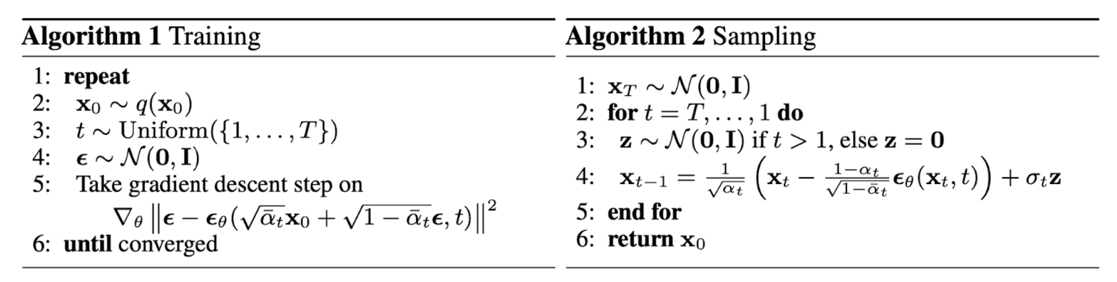
训练过程:
- 采样一个$x_0$
- 任选一个时间t
- 随机采样一个高斯噪声$\epsilon$
- 计算损失函数的梯度,更新参数$\theta$
采样过程:
- 采样一个高斯噪声$x_T$
- 从时间T开始,每一步采样一个高斯噪声z,利用重参数化,得到上一步的$x_{t-1}$,重复T次,最终得到生成的$x_0$
注意这里还没有给出$\epsilon_\theta(x_t, t)$的网络结构,DDPM使用U-Net作为其网络结构(后面会具体展开)
2.5. 小结
简单来说,扩散模型的前向扩散过程都是定义好的马尔可夫链,每一步都需要使用重参数化技巧来添加噪声,这里每一步的后验分布的参数都是预定义好的。反向扩散过程就是用噪声生成原始图片的过程,和VAE类似,用分布$p_\theta(x_{t-1}|x_t)$来拟合真实的后验分布$q(x_{t-1}|x_t)$,所以生成过程最重要的就是训练出合适的分布来拟合,通过VLB和重参数化的技巧,最终可以把训练过程看成给一个高斯噪声,拟合成前向扩散的噪声。这里的网络结构一般使用的是U-Net
3. 一些技巧和主要网络结构
3.1. $\beta_t$和$\Sigma_\theta$的取值
关于$\beta_t$的取值,DDPM的做法是$\beta_1=10^{-4}$到$\beta_T=0.02$线性取值,这样的扩散模型取得的效果不算最好,Improved DDPM提出了一种新的取值方法:
\begin{equation}
\beta_t = \text{clip}(1-\frac{\bar{\alpha}_t}{\bar{\alpha}_{t-1}}, 0.999) \quad\bar{\alpha}_t = \frac{f(t)}{f(0)}\quad\text{where }f(t)=\cos\Big(\frac{t/T+s}{1+s}\cdot\frac{\pi}{2}\Big)
\end{equation}
关于$\Sigma_\theta$的取值方法,DDPM采用固定的$\Sigma_\theta$(不学习),可以取$\beta_t$或者$\tilde{\beta_t}=\frac{1 - \bar{\alpha_{t-1}}}{1 - \bar{\alpha_t}} \cdot \beta_t$,Improved DDPM采用可学习的$\Sigma_\theta$参数,利用线性插值的方法:
\begin{equation}
\boldsymbol{\Sigma}_\theta(\mathbf{x}_t, t) = \exp(\mathbf{v} \log \beta_t + (1-\mathbf{v}) \log \tilde{\beta}_t)
\end{equation}
由于损失函数中没有关于$\Sigma_\theta$的梯度,所以需要对损失函数进行一点更改
3.2. 加速扩散模型采样的技巧
DDPM的作者对比了扩散模型和其他生成模型的生成速度,发现DDPM的生成速度远小于其他生成模型,有一些加速模型采样的技巧:
- 缩短采样步骤,比如每隔T/S步才采样一次
- DDIM论文里提出的技巧,在采样过程中只需要采样一个子集的步骤便可做生成
- Latent Diffusion Model论文提出让扩散过程在隐空间中进行,而不是在像素空间中进行,这样可以让训练代价更小,推断过程更快,后续会整理LDM论文
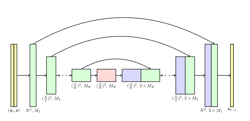
3.3. U-Net
很多扩散模型的噪声网络结构都是基于U-Net,U-Net的网络结构如下图:
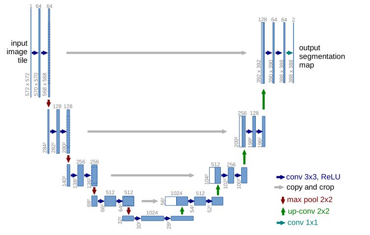
模型可以分为两个部分,左边用于特征的抽取,右边部分用于上采样,由于网络结构酷似字母U而得名。U-Net网络结构又可以看成AutoEncoder的结构,它的bottleneck就是中间的低纬度特征表示,U-Net要保证输出的噪声和输入的噪声有相同的维度,是一个自回归模型。DDPM使用的是PixelCNN++的backbone,也就是基于Wide Resnet的U-Net,也就是说encoder和decoder之间是残差连接,输入$x_t$返回噪声(残差思想)
4. 条件生成
条件生成就是conditioned generation,通过输入额外的conditioning information来生成图片,比如一段提示词或者生成图片的类别
4.1. Classifier Guided Diffusion
博客上讲解的关于classifier guidance的部分不太详尽,于是我去翻看了Classifier Guidance的论文Diffusion Models Beat GANs:
classifier guidance的思路来源于GAN模型的条件生成,将这种条件生成应用于扩散模型后,发现效果非常好。作者提出可以训练一个分类器$p_\phi(y|x_t, t)$,然后把$\nabla_{x_t} \log p_\phi\left(y \mid x_t, t\right)$的加到总的梯度公式里面,来指导扩散模型采样的过程偏向于生成类别为y的图片
没有classifier guidance之前的反向扩散分布函数为: $p_\theta(x_t|x_{t+1})$,但是有了classifier guidance之后,反向扩散的后验分布函数变成了:
\begin{equation}
p_{\theta, \phi}(x_t|x_{t+1}, y) = Zp_\theta(x_t|x_{t+1})p_\phi(y|x_t)
\end{equation}
其中Z是正则化的常数,接下来我们需要化简上面这个公式,首先我们知道$p_\theta(x_t|x_{t+1})$本质上就是正态分布:
\begin{equation}
p_\theta(x_t|x_{t+1})=\mathcal{N}(\mu, \Sigma)
\end{equation}
然后我们对$log_\phi p(y|x_t)$在$x=\mu$处进行泰勒展开:
\begin{equation}
\begin{aligned}
\log p_\phi(y \mid x_t) & \approx log p_\phi (y \mid x_t) \mid _{x_t=\mu}+(x_t-\mu)\nabla_{x_t}logp_\phi(y \mid x_t)\mid _{x_t=\mu} \\
&=(x_t-\mu)g+C_1\\
\end{aligned}
\end{equation}
这里$g=\nabla_{x_t}logp_\phi(y \mid x_t)\mid _{x_t=\mu}$
\begin{equation}
\begin{aligned}
\log \left(p_\theta\left(x_t \mid x_{t+1}\right) p_\phi\left(y \mid x_t\right)\right) & \approx-\frac{1}{2}\left(x_t-\mu\right)^T \Sigma^{-1}\left(x_t-\mu\right)+\left(x_t-\mu\right) g+C_2 \\
&=-\frac{1}{2}\left(x_t-\mu-\Sigma g\right)^T \Sigma^{-1}\left(x_t-\mu-\Sigma g\right)+\frac{1}{2} g^T \Sigma g+C_2 \\
&=-\frac{1}{2}\left(x_t-\mu-\Sigma g\right)^T \Sigma^{-1}\left(x_t-\mu-\Sigma g\right)+C_3 \\
&=\log p(z)+C_4, z \sim \mathcal{N}(\mu+\Sigma g, \Sigma)
\end{aligned}
\end{equation}
那么反向扩散过程就可以看成均值为$\mu+\Sigma g$,方差为$\Sigma$的正态分布,那么我们有以下采样算法:
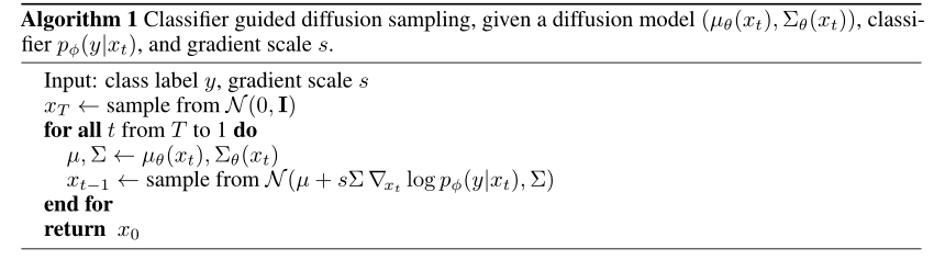
另一种思路是修改正态分布中的噪声函数,原本的梯度为:
\begin{equation}
\nabla _{x_t} log p_\theta (x_t) = - \frac{1}{\sqrt{1-\overline{\alpha_t}}} \epsilon_\theta (x_t)
\end{equation}
修改反向扩散函数后的梯度为:
\begin{equation}
\begin{aligned}
\nabla _{x_t} log (p_\theta (x_t) p_\phi (y \mid x_t)) &= \nabla _{x_t} log p_\theta (x_t) + \nabla _{x_t} log p_\phi (y \mid x_t) \\
&= - \frac{1}{\sqrt{1-\overline{\alpha_t}}} \epsilon_\theta (x_t) + \nabla _{x_t} log p_\phi (y \mid x_t)
\end{aligned}
\end{equation}
那么根据梯度,我们可以定义一个新的噪声预测函数$\hat{\epsilon}$:
\begin{equation}
\hat{\epsilon(x_t)} := \epsilon_\theta(x_t) - \sqrt{1-\overline{\alpha_t}} \nabla _{x_t} log p_\phi(y \mid x_t)
\end{equation}
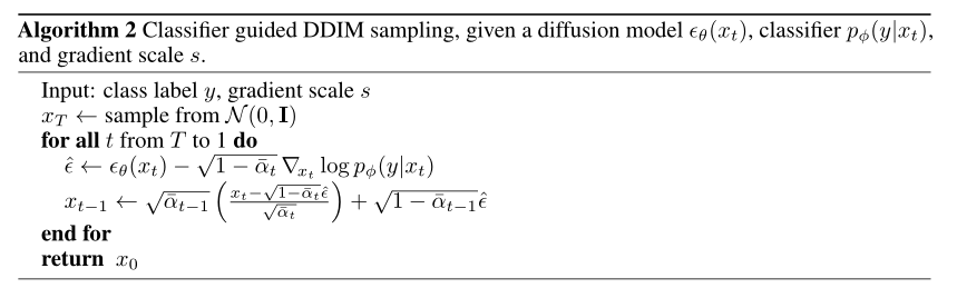
该方法对应的算法为:
4.2. Classifier-Free Guidance
上一小节提到的classifier guidance的技巧是需要单独使用一个分类器(参与训练或者不参与训练的情况都有)来获得$x_t$的类别,根据不同的class可以使用不同的分类器,比如resnet可以进行图片类别的guidance,CLIP可以进行文本的guidance等等。如果我们没有这个单独的分类器,我们也可以利用classifier-free guidance的技巧来实现条件生成,同样地,为了更详尽地了解这个技巧,我去翻看了GLIDE论文中关于classifier-free guidance的介绍
classifier-free guidance并不需要模型去单独给出一个分类器,而是将条件生成与非条件生成都用同一个函数表示,即$\epsilon(x_t\mid y)$,如果我们希望这个函数表示非条件生成,那么我们只需要将y替换成空集即可,在训练过程中,我们以相同的概率随机替换y为空集。采样时,反向扩散函数为$\epsilon_\theta(x_t \mid y)$和$\epsilon_\theta(x_t \mid \emptyset)$的线性插值:
\begin{equation}
\hat{\epsilon_\theta}(x_t \mid y)=\epsilon_\theta(x_t\mid \emptyset) + s \cdot (\epsilon_\theta(x_t\mid y)-\epsilon_\theta(x_t\mid \emptyset))
\end{equation}
式子中的s是guidance scale,s越大代表生成的图片越靠近y,guidance-free的技巧出现后,大家发现它的效果非常好,于是后续的模型基本上都运用了该技巧,比如GLIDE、DALLE2、Imagen
4.3. Scale up Generation Resolution and Quality
为了生成更高质量和更高分辨率的图片,可以将扩散模型与超分辨率的技术相结合,论文Cascaded Diffusion Model中提出用层级式的扩散模型来做图片的超分辨率生成,模型的结构如下图:
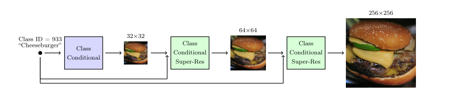
模型由三个子模型组成,分别是一个基础的扩散模型和两个超分辨率扩散模型,注意这里的每个子模型都需要输入类别,超分辨率子模型还需要输入上一个子模型的低分辨率结果,这些子模型都是conditional的。超分辨率扩散模型与普通的扩散模型的区别是损失函数和反向扩散函数不同,具体来说就是U-Net的结构不同,超分辨率的U-Net的输出维度比输入维度要大,而且输入为低分辨率的图片、高分辨率的图片、类别:
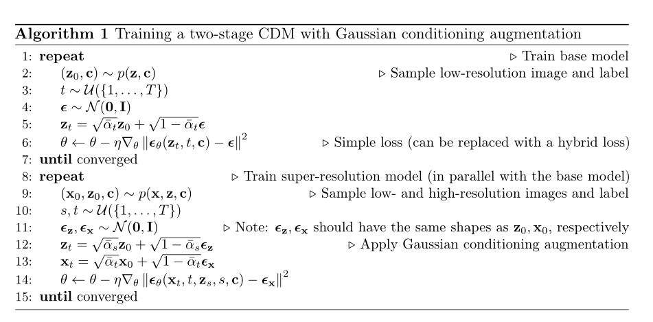
一个two-stage的cascaded模型的训练算法为:
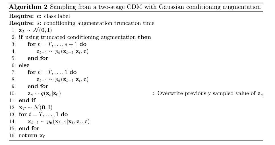
一个two-stage的cascaded模型的采样算法为:

Comments